
Welcome to part 3. In the previous two parts (Part1 and Part 2) we saw how to read the geonames database CSV file and how to use Logstash to send the data to Elasticsearch. We adjusted the Elasticsearch index mapping to reflect the proper data types - especially for the latitude and longitude position of the individual data points.
Before we continue, make sure you started your Elasticsearch and Kibana instances. Go to http://localhost:5601 in your Web browser.
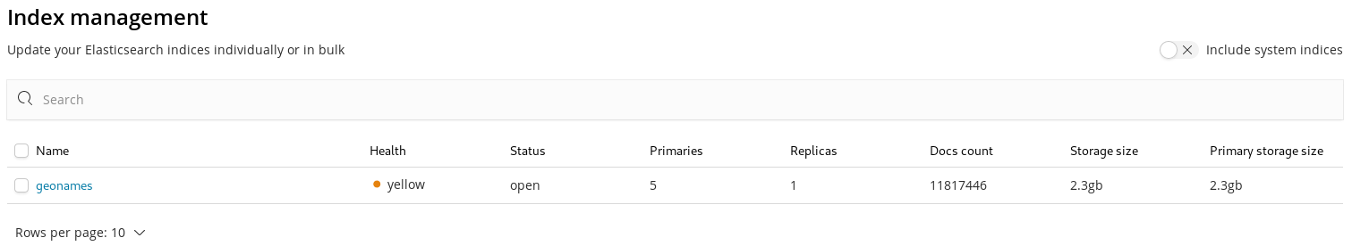
We have created an index with 10000 data points in Elasticsearch. But meanwhile I have deleted this one and imported the complete geonames CSV file - around 12 million data points. I named the index "geonames".
Before we continue, make sure you started your Elasticsearch and Kibana instances. Go to http://localhost:5601 in your Web browser.
We have created an index with 10000 data points in Elasticsearch. But meanwhile I have deleted this one and imported the complete geonames CSV file - around 12 million data points. I named the index "geonames".
The next things we have to do is to create a Kibana "Index Pattern". By doing this, one can actually use multiple Elasticsearch indexes for the same visualizations. E.g. one could create an index per day or per month. This can be an advantage with changing schemas but also for cleaning up (deleting) data. In this case though we have only one Elasticsearch index available. Creating an "Index Pattern" also allows us to steer the formatting of the individual fields, e.g. how dates are displayed.
To create an index pattern click on the "Management" link on the lower left-hand side of the browser window and then under the "Kibana" section, click on "Index Patters". If you have not defined any index pattern so far, you will see a page which allows you to define a first one:
To create an index pattern click on the "Management" link on the lower left-hand side of the browser window and then under the "Kibana" section, click on "Index Patters". If you have not defined any index pattern so far, you will see a page which allows you to define a first one:
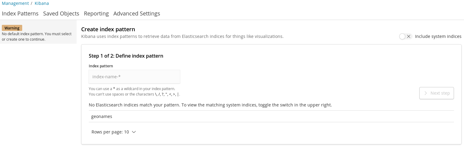
In the textbox labeled "Index Pattern" enter: geonames. This is the name of the Elasticsearch index we created. Then click on "Next Step". On the following page select "I don't want to use the Time Filter" from the dropdown labeled "Time Filter field name".
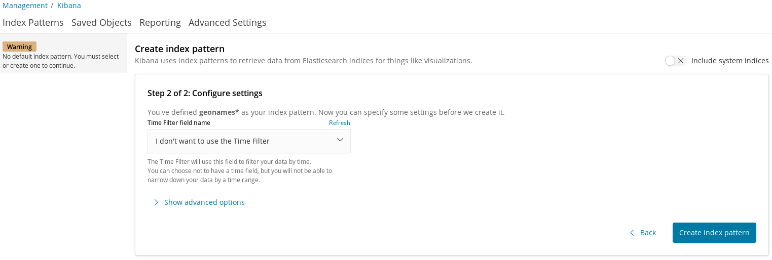
Note: In Kibana date and time can be used to visualize data relatively to the moment when events happened. But in this data set we really only have the "modification date". This is not so interesting like say e.g. the event date and time of people clicking on web pages to order products. So for this showcase we will ignore date and time.
Finally, click on "Create index pattern". We are now ready to create visualizations on top of this.
On the left side of the browser window click on "Visualize" and then click on the big blue "plus" button. The page displays the different visualization types available. Select "Coordinate Map" under the section "Maps". We will use this to visualize the latitude and longitude position of all points in the data set. You are now asked which index pattern to use - select "geonames", the pattern we just created.
You should now have an empty map displayed on the right side of the browser window.
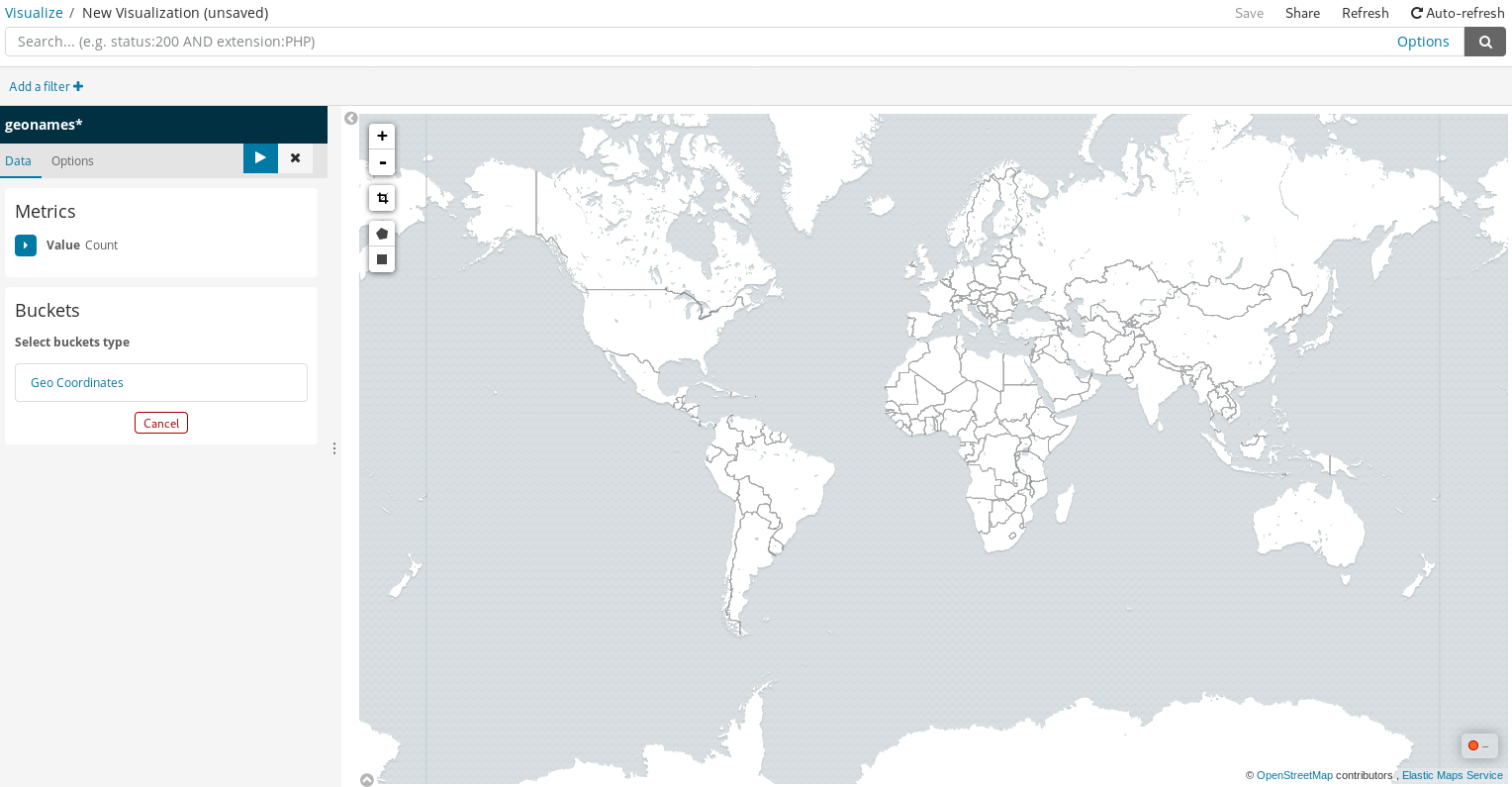
On the left side under "Metrics", you see that "count" is selected as aggregation method. Under "Buckets" nothing is selected - this is why we don't see anything on the map.
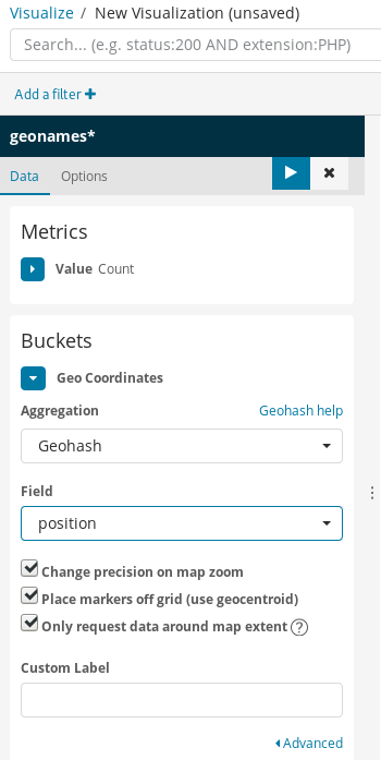
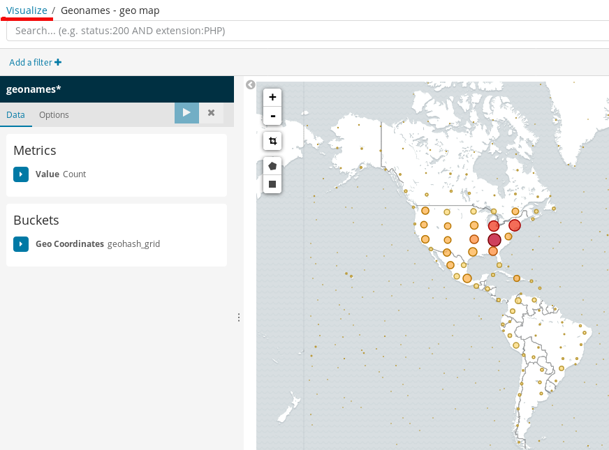
To change this, under "Buckets", click on "Geo Coordinates" then "Geohash" and then select the field that carries the latitude and longitude positions of our data. In our case this is the field "position". It should look like this:
To change this, under "Buckets", click on "Geo Coordinates" then "Geohash" and then select the field that carries the latitude and longitude positions of our data. In our case this is the field "position". It should look like this:
Now click on the blue "play" button. The map will now be populated.
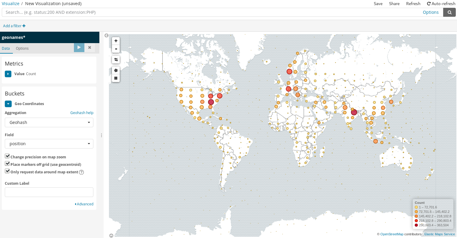
You can use the plus/minus buttons or draw a rectangle to zoom in to a certain area. And of course you can move the map by dragging it.
On the top right on the visualization there is a link labeled "Save". Click here to save the visualization by giving it an appropriate name.
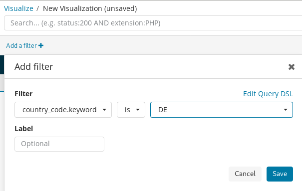
Click on "Add a filter" and select e.g. the field "country_code.keyword" then "is" (equals) and then "DE" (for Germany).
On the top right on the visualization there is a link labeled "Save". Click here to save the visualization by giving it an appropriate name.
Click on "Add a filter" and select e.g. the field "country_code.keyword" then "is" (equals) and then "DE" (for Germany).
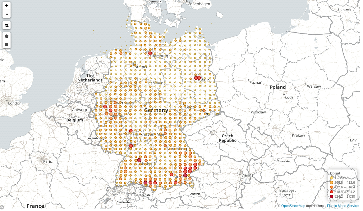
Then click on "Save". The map will be updated accordingly. if you center the map ("Fit data bounds - third icon from the top on the map display) and zoom in a little bit, you see a more detailed view on the available data for Germany.
You can add more filters. Or you can use the search bar on top to search for something. E.g. if you simply add "Munich" in the search bar, then all available data/fields will be searched for this word and displayed on the map.
You can also enter something like: feature_name.keyword : "water mill" to get all water mills displayed. In the search bar you can use "AND" and "OR" to combine search conditions according to your needs.
Make sure you save your visualization. I have saved it without any filters. We will now create another visualization - a bar chart. On the current visualization click on "Visualize" in the upper left hand corner - as shown below, to add a new one.
Then click on the blus "plus" button, select "Vertical Bar" as visualization type and select "geonames" as index pattern. You will get a page with one big vertical bar showing the total count over all available data.
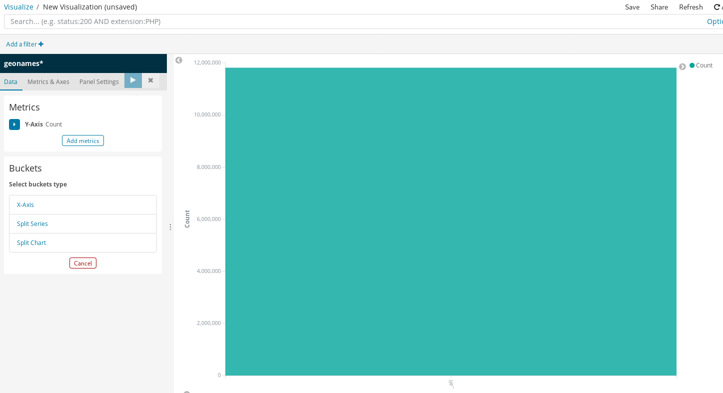
Under "Buckets" click on "X-Axis", then under "Aggregations" select "Terms" and select the field "feature_name.keyword" and then click the blue "play" button. The barchart will now show the total number of data points available devided by their feature name. Per default only the top 5 are shown. You can adjust this on the left side by entering a different value in the field labeled "Size" - e.g. change it to "10".
Now save this visualization as e.g. "Geonames - counts per feature_name".
Next, click on "Dashboard" on the left side of the browser window and then click on the blue button. You will get this:
Now save this visualization as e.g. "Geonames - counts per feature_name".
Next, click on "Dashboard" on the left side of the browser window and then click on the blue button. You will get this:
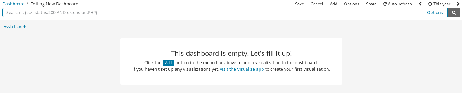
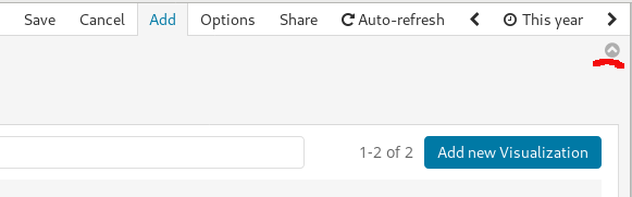
Click on "Add" on the upper left and you will see a list of available visualizations - the two that we created and saved. Click on the names of both of them and they are added to the dashboard. You can now collapse the list of the visualizations by clicking on the collapse arrow (pointing upwards - see below).
Out first dashboard now looks like this:
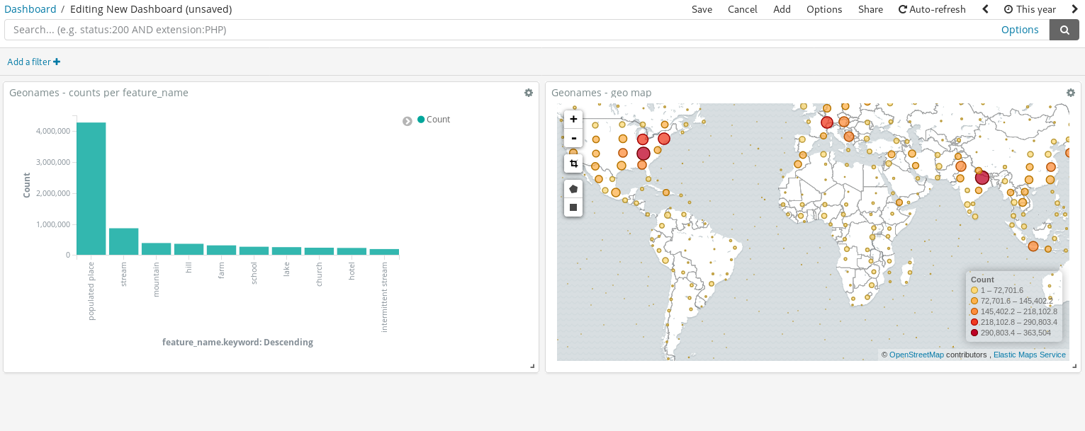
Go ahead and save it with an appropriate name. As is, the dashboard shows both on the map and in the barchart (top 10) the total number of data points without any filters (if you have not defined a filter in the visualization itself).
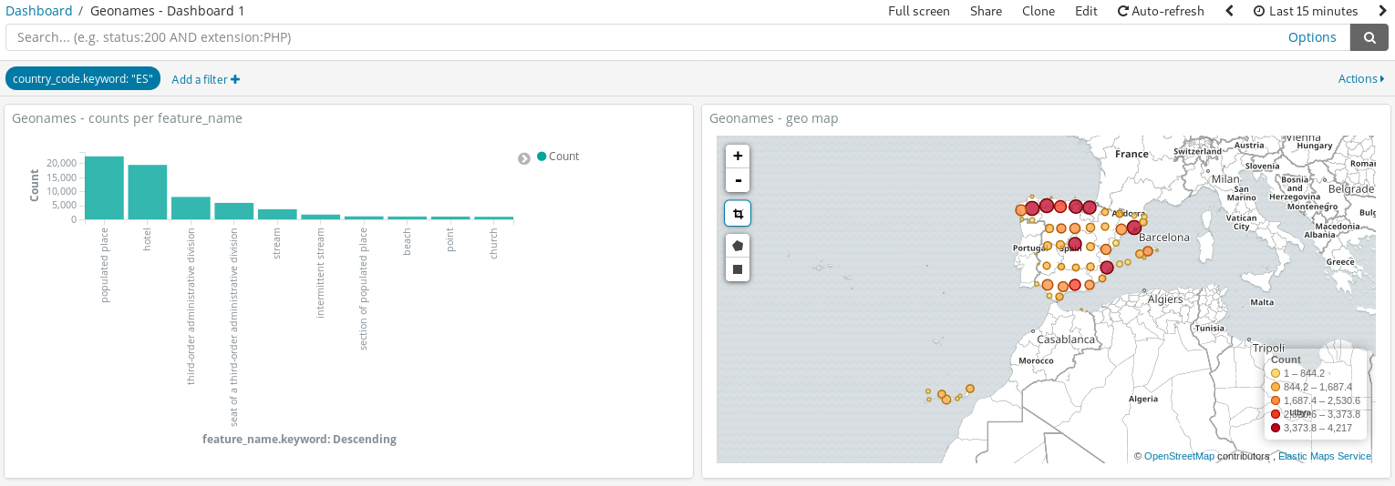
You can now add a filter like we did before. E.g. add a filter to select only the data points in Spain (country_code.keyword is ES). Once the filter is saved the barchart and the geomap are updated. Again you can fit the data bounds or zoom in/out.
Or you could simply draw a rectangle (last button on the geomap, on the left side) to select an area and then an automatic filter for the selected area will be created and the barchart is updated accordingly.
Here are the other parts:
So this is the first dashboard we create on top of the geonames data. There are many more visualizations available - go and try them out. You can combine them into one or multiple dashboards.
Hope you enjoyed this three-part blog about Logstash, Elasticsearch and Kibana. Make sure you come back frequently to read more articles about this amazing technology.
Carpe Diem
- https://datamelt.weebly.com/blog/elasticsearch-a-practical-example-part-1
- https://datamelt.weebly.com/blog/elasticsearch-a-practical-example-part-2
So this is the first dashboard we create on top of the geonames data. There are many more visualizations available - go and try them out. You can combine them into one or multiple dashboards.
Hope you enjoyed this three-part blog about Logstash, Elasticsearch and Kibana. Make sure you come back frequently to read more articles about this amazing technology.
Carpe Diem
 RSS Feed
